Tutorial 1
This tutorial shows an example of basic HydroVisE configuration and deployment given in example folder in HydroVisE GitHub repository. In this example tutorial, we assume that user has Google Chrome and wants to deploy HydroVisE for visualizing their data on web-browser.
The objective of this tutorial is to describe basics of HydroVisE data organization, configuration, and deployment.
First, we need a web-server.
For this example, we use Chrome web-server extension that can be installed from here.
Click on Add to Chrome

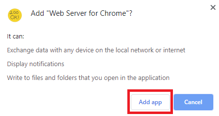
Click on Add app
If you open this extension, a window will be shown as below. Choose the folder that you want to extract HydroVisE zip folder.

Let's download HydroVisE code's Zip file and unzip its content to web-server's root location.
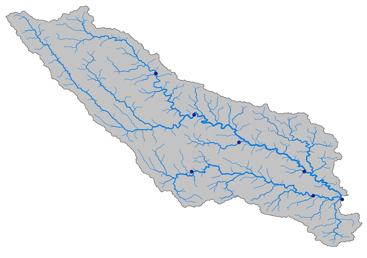
Let us start from an example of hydrologic model simulation and performance evaluations. For this example, we have selected Turkey River watershed located in North-East of the state of Iowa. As shown in the figure below, there are 7 USGS streamflow gauges inside this basin.
 |
|---|
| Domain of interest: Turkey River basin - Blue dots show the locations of USGS streamflow observations in this basin. River network is shown as light blue lines with different size that correspond to horton order. |
Let's assume that user is interested in visualizing the streamflow data corresponding to each location shown in figure above. These locations are specified by mapMarkers in HydroVisE config file. mapMarkers is a geoJSON file that contains geographic location of the markers along with CRS (Coordinate Reference System) that defines the georeference of the features inside the geometry collection. In this example, we use a geoJSON file as shown below:
{
  "type": "FeatureCollection",
  "name": "mapMarkers",
  "crs": { "type": "name", "properties": { "name": "urn:ogc:def:crs:OGC:1.3:CRS84" } },
  "features": [
    { "type": "Feature", "properties": { "lid": 399598, "usgs_id": "05412340", "usgs_name": "Volga River at Fayette (05412340)", "area": 336.6987, "lat": 42.844139, "lon": -91.818167 }, "geometry": { "type": "Point", "coordinates": [ -91.81817, 42.84414 ] } },
    { "type": "Feature", "properties": { "lid": 399711, "usgs_id": "05412400", "usgs_name": "Volga River at Littleport (05412400)", "area": 909.08649, "lat": 42.753875, "lon": -91.369025 }, "geometry": { "type": "Point", "coordinates": [ -91.36902, 42.75388 ] } },
    { "type": "Feature", "properties": { "lid": 418967, "usgs_id": "05411900", "usgs_name": "Otter Creek at Elgin (05411900)", "area": 0.0, "lat": 42.952512, "lon": -91.643016 }, "geometry": { "type": "Point", "coordinates": [ -91.64302, 42.95251 ] } },
    { "type": "Feature", "properties": { "lid": 483619, "usgs_id": "05411600", "usgs_name": "Turkey River at Spillville (05411600)", "area": 458.42823, "lat": 43.207278, "lon": -91.950333 }, "geometry": { "type": "Point", "coordinates": [ -91.95033, 43.20728 ] } },
    { "type": "Feature", "properties": { "lid": 434365, "usgs_id": "05411850", "usgs_name": "Turkey River near Eldorado (EDRI4-05411850)", "area": 1667.95356, "lat": 43.054188, "lon": -91.809098 }, "geometry": { "type": "Point", "coordinates": [ -91.8091, 43.05419 ] } },
    { "type": "Feature", "properties": { "lid": 434478, "usgs_id": "05412020", "usgs_name": "Turkey River above French Hollow Cr at Elkader (EKDI4-05412020)", "area": 2359.48089, "lat": 42.843485, "lon": -91.401277 }, "geometry": { "type": "Point", "coordinates": [ -91.40128, 42.84349 ] } },
    { "type": "Feature", "properties": { "lid": 434514, "usgs_id": "05412500", "usgs_name": "Turkey River at Garber (GRBI4-05412500)", "area": 4032.61443, "lat": 42.739988, "lon": -91.261799 }, "geometry": { "type": "Point", "coordinates": [ -91.2618, 42.73999 ] } }
  ]
}
A user might be interested in visualizing multiple time-series associated with each location for multiple years. Folder structure for the time-series data could look like below:
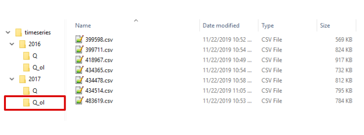
Folders and subfolders are organized with year, variable name and comID. In this example, file names are comID's that relate the spatial location to data. The comID name correspond to lid inside mapMarkers geoJSON file.
timeseries/year/var_name/comID.csv
NOTE: In this example, we have organized the data with folders and subfolders. But this is not a requirement for HydroVisE as long as the file path template string is defined properly.
In this example streamflow timeseries data are provided as CSV files with header names that are used in traces object inside config file.
dt,Q
2016-01-01 00:00:00,5.295
2016-01-01 00:15:00,5.295
2016-01-01 00:30:00,5.210
2016-01-01 00:45:00,5.210
.
.
.
2016-12-31 23:45:00,6.350
First column dt corresponds to datetime with YYYY-MM-DD HH:mm:SS.
Second column corresponds to variable name same as folder name shown in folder structure Q.
Let's call our config filename as "testconfig.json" and put it in the example folder on the web-server.
{
"page":{
"title": "HydroVisE - Tutorial 1"
},
"map": {
"center": [
43.041,
-91.57
],
"defaultZoom": 10,
"maxZoom": 15,
"basemapList": {
"default": {
"id": "light_all",
"url": "http://{s}.basemaps.cartocdn.com/light_all/{z}/{x}/{y}.png",
"attribution": "© <a href=\"http://www.openstreetmap.org/copyright\">OpenStreetMap</a> contributors, © <a href=\"https://carto.com/attributions\">CARTO</a>",
"subdomains": "abcd"
}
},
"geoSearch": true
},
"data_part": {
"min_val": 2016,
"max_val": 2017,
"step": 1,
"initial": 2016
},
"traces": {
"t1": {
"prod": "Q",
"x_name": "dt",
"y_name": "Q",
"modEnabled": 0,
"dynamic": 0,
"ensemble": 0,
"template": {
"var": [
"yr",
"comID"
],
"path_format": "example/timeseries/{0}/Q/{1}.csv"
},
"style": {
"type": "scattergl",
"mode": "lines",
"name": "USGS",
"line": {
"width": 2,
"color": "black"
}
}
},
"t2": {
"prod": "Q_ol",
"x_name": "dt",
"y_name": "Q",
"modEnabled": 0,
"dynamic": 0,
"ensemble": 0,
"template": {
"var": [
"yr",
"comID"
],
"path_format": "example/timeseries/{0}/Q_ol/{1}.csv"
},
"style": {
"type": "scattergl",
"mode": "lines",
"name": "Open Loop",
"line": {
"color": "blue"
}
}
}
},
"mapMarkers": {
"fnPath": "example/vectors/mapMarkers.geojson",
"comIDName": "lid",
"geomType":"point",
"onEachFeature":{
"click": "clickFeature"
},
"plotTitle": {
"template": {
"var": ["usgs_name","area"],
"format": "{0}<br>Area: {1} km<sup>2</sup>"
}
},
"tooltip": {
"template": {
"var": [
"usgs_name",
"area",
"metricName",
"metric"
],
"format": "<b>USGS Name:</b><br> {0}<br><b>Area: </b>{1} km<sup>2</sup>"
}
}
},
"controls": {
"baseMapType": {
"v1": {
"var_id": "light_all",
"var_name": "Light",
"onEvent": "basemap_changer",
"selected": 1
}
}
},
"plotlyLayout": {
"margin": {
"l": 80,
"r": 80,
"b": 70,
"t": 50,
"pad": 1
},
"titlefont": {
"size": 16,
"color": "black"
},
"legend": {
"x": 0,
"y": 1,
"traceorder": "normal",
"font": {
"size": 14,
"color": "#000"
},
"bgcolor": "rgba(255,255,255,0.90)",
"bordercolor": "#000000",
"borderwidth": 1,
"orientation": "h"
},
"xaxis": {
"titlefont": {
"size": 18,
"color": "#1c1c1c"
},
"tickfont": {
"size": 18,
"color": "black"
},
"type": "date"
},
"yaxis": {
"title": "Q (m3/s)",
"titlefont": {
"size": 18,
"color": "#1c1c1c"
},
"tickfont": {
"size": 18,
"color": "black"
},
"autorange": true,
"rangemode": "tozero",
"hoverformat": ".1f"
},
"plot_bgcolor": "#fff",
"paper_bgcolor": "#eee",
"hovermode": "closest",
"updatemenus": [
{
"buttons": [],
"direction": "left",
"pad": {
"r": 10,
"t": 10
},
"showactive": true,
"type": "buttons",
"x": 0,
"xanchor": "left",
"y": 1.15,
"yanchor": "top"
}
],
"initMD": "-04-01 00:00:00",
"finalMD": "-11-01 00:00:00",
"displayModeBar": true
},
"mapLayers": {
"IACounties.geojson": {
"fnPath": "example/vectors/mapLayers/IACounties.geojson",
"fn": "IACounties.geojson",
"var_name": "IA Counties",
"onEvent": "toggLyrStd",
"selected": false
}
},
"customBaseMap": {
"url": "example/vectors/customBaseMap.geojson.gz",
"colors": {
"3": "#00e4ff",
"4": "#00c5ff",
"5": "#00acff",
"6": "#018eff",
"7": "#007dff",
"8": "#007bff",
"9": "#0055ff",
"10": "#000000",
"11": "#321321"
},
"propoertyName": "h_order",
"name" : "River Network"
}
}Try it yourself!
Here is what this configuration setup for HydroVisE looks like:
Now, let's say we have values that we can use for color-coding the markers and navigating over these values. For example, these values could be a hydrologic model's performance metrices.
We can enable control elements for navigating over marker attributes (metrices) and variables (simulation types) by adding two objects (described in Configuration).
First, we need to defvine the data source for marker Attributes inside mapMarkers object in the config file.
Let's add this object to mapMarkers object.
"markerAttrs": {
      "template": {
        "var": [],
        "path_format": "example/vectors/markerAttrs.csv"
      },
      "comID": "lid"
    }
For this example, we use lid column as comID to be consistent. The CSV content is shown below. In this case, metrices for performance evaluations. A CSV file is provided to the config:
year,prod,correlationcoefficient,kge,nashsutcliffe,lid,Area,Slope,t_trav,nRMSE,nMAE,timing,norm_bias,ppd,pt_change_vol
2016,Q_ol,0.633,0.387,0.358,399598.000,336.699,0.055,14.230,0.009,0.006,0.000,0.197,-0.512,23.594
2016,Q_ol,0.877,0.832,0.735,399711.000,909.086,0.148,38.310,0.009,0.005,2.000,0.079,0.050,10.563
2017,Q_ol,0.896,0.856,0.795,399711.000,909.086,0.148,38.310,0.016,0.007,2.000,0.045,-0.203,9.426
2016,Q_ol,0.919,0.578,0.773,483619.000,458.428,0.067,22.500,0.025,0.012,0.000,-0.146,-0.379,-27.398
2017,Q_ol,0.591,0.511,0.112,483619.000,458.428,0.067,22.500,0.011,0.007,0.000,0.269,-0.238,26.640
2016,Q_ol,0.869,0.436,0.610,434365.000,1667.954,0.080,43.980,0.028,0.013,1.000,-0.176,-0.531,-29.267
2017,Q_ol,0.682,0.631,0.409,434365.000,1667.954,0.080,43.980,0.012,0.008,2.000,0.129,-0.240,14.206
2016,Q_ol,0.872,0.555,0.680,434478.000,2359.481,0.116,70.140,0.019,0.009,2.000,-0.162,-0.211,-23.062
2017,Q_ol,0.616,0.577,0.314,434478.000,2359.481,0.116,70.140,0.011,0.007,8.000,0.107,-0.286,9.210
2016,Q_ol,0.860,0.657,0.707,434514.000,4032.614,0.139,80.270,0.013,0.006,3.000,-0.110,-0.184,-12.971
2017,Q_ol,0.810,0.768,0.616,434514.000,4032.614,0.139,80.270,0.010,0.006,2.000,0.121,-0.065,12.561
year,prod which is variable name (or product name), lid (comID) are required for selecting marker attributes for color coding. At least one attributes should be provided in this CSV file for colorcoding the markers. Here is a table that describes the markerAttributes given above:
| var_id | Description |
|---|---|
| year | Corresponding year for the metric |
| prod | Name of the product |
| lid | LinkID as an identifier for comID |
| correlationcoefficient | Correlation Coefficient |
| kge | Kling-Gupta Efficiency |
| nashsutcliffe | Nash-Sutcliff Efficiency |
| Area | Upstream Area (km2) |
| Slope | Mean Slope of the basin |
| t_trav | Travel time (hr) |
| nRMSE | Normalized Root mean Squred Error |
| nMAE | Normalized Mean Absolute Error |
| timing | Timing difference of the peak |
| norm_bias | Normalized Basia |
| ppd | Percent peak difference |
| pt_change_vol | Percent volume difference |
Define metrices/attributes for color-coding. We have only one product (prod) that has associated marker attributes. Therefore, here is an addition to controls object.
"prod":{
  "Q_ol": {
        "var_id": "Q_ol",
        "var_name": "Open loop",
        "onEvent": "select_sim_type",
        "selected": 1
      }
}
Add control elements and color palettes for each attribute of interest from markerAttrs CSV file using this addition to controls in config file.
"controls":{
  "markerAttrs": {
      "kge": {
        "var_id": "kge",
        "var_name": "KGE",
        "onEvent": "selectMetric",
        "selected": 1,
        "colorPalette": ["#ffffcc","#ffeda0","#fed976","#feb24c","#fd8d3c","#fc4e2a","#e31a1c","#bd0026","#800026"],
        "nBins": 11,
        "method": "equidistant",
        "range": [-0.1, 1]
      },
      "correlationcoefficient": {
        "var_id": "correlationcoefficient",
        "var_name": "Correlation",
        "onEvent": "selectMetric",
        "selected": 0,
        "colorPalette": ["#003a00", "#20600a", "#438815", "#6cb23e", "#99dc6c", "#fbb9e8", "#f67bcd", "#dd439b", "#af1d6b", "#7a0040"],
        "nBins": 10,
        "method": "equidistant",
        "range" :[-1, 1],
		"decimals": 2
      }
    },
    "prod":{
      "Q_ol": {
        "var_id": "Q_ol",
        "var_name": "Open loop",
        "onEvent": "select_sim_type",
        "selected": 1
      }
    }
}
Let's say user wants to see the selected metric name and the value when hovering on the location. This can be done by modifying the tooltip object inside markerAttrs as follows:
Previous tooltip object looks like this:
"tooltip": {
  "template": {
    "var": [
      "usgs_name",
      "area"
    ],
    "format": "<b>USGS Name:</b><br> {0}<br><b>Area: </b>{1} km<sup>2</sup>"
  }
}
After adding markerAttrs file shown above, we can add metric name and value to tooltip by modifying the tooltip object.
"tooltip": {
  "template": {
    "var": [
      "usgs_name",
      "area",
      "metricName",
      "metric"
    ],
    "format": "<b>USGS Name:</b><br> {0}<br><b>Area: </b>{1} km<sup>2</sup><br><b>{2}:</b> {3} "
  }
}
Note that if some locations do not have a value for the selected attribute for any reason, the corresponding location will neither be color-coded nor included in the tooltip.
![]()
- Tutorial 1
- More tutorials will be added soon
- Real-time and Historical USGS Streamflow Viewer
- Sensor and Satellite-based Soil Moisture Visualization
- Satellite-based Soil Moisture Assimilation in Hydrologic Model
- Hydrologic Model Streamflow Forecasts Visualization