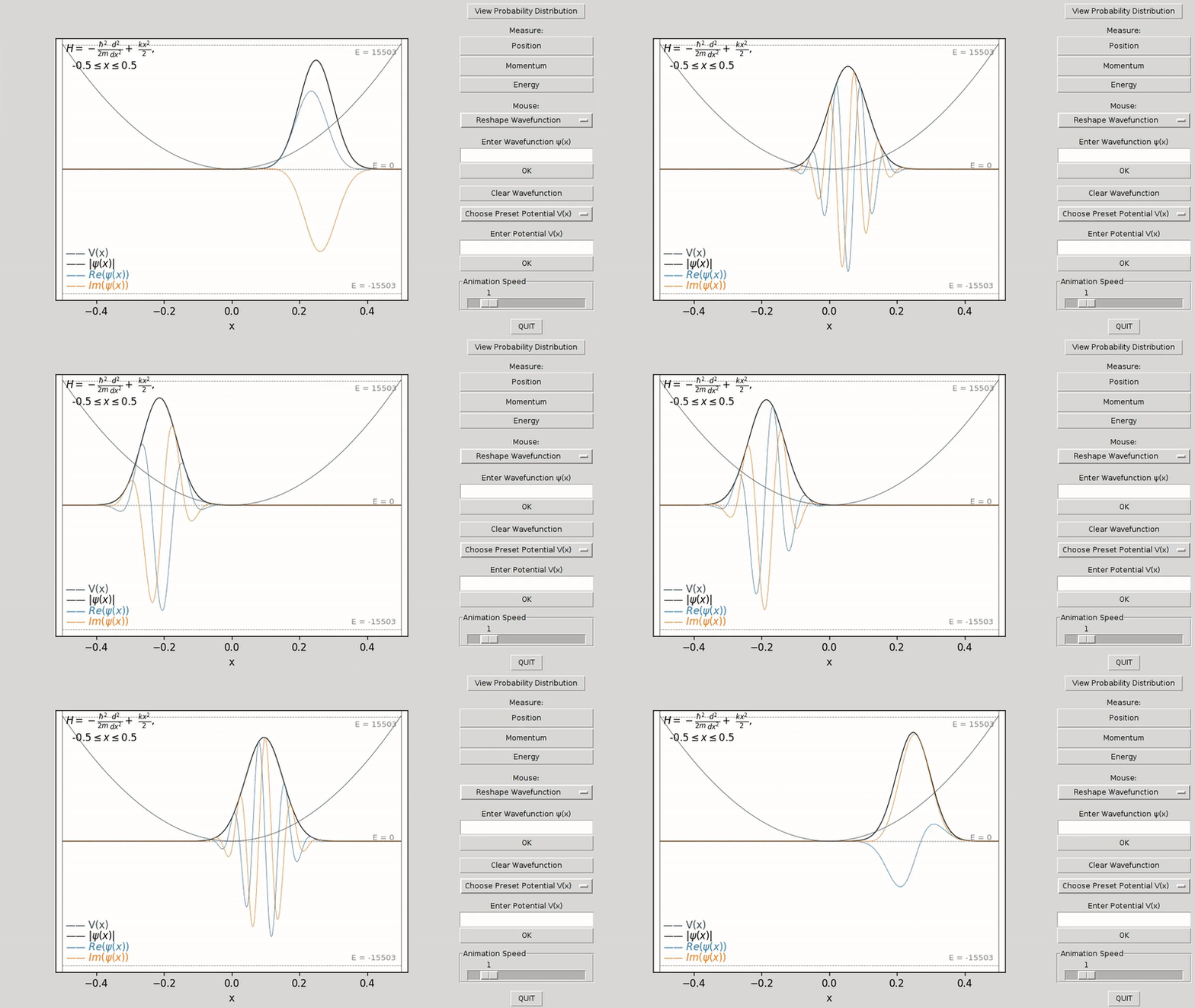
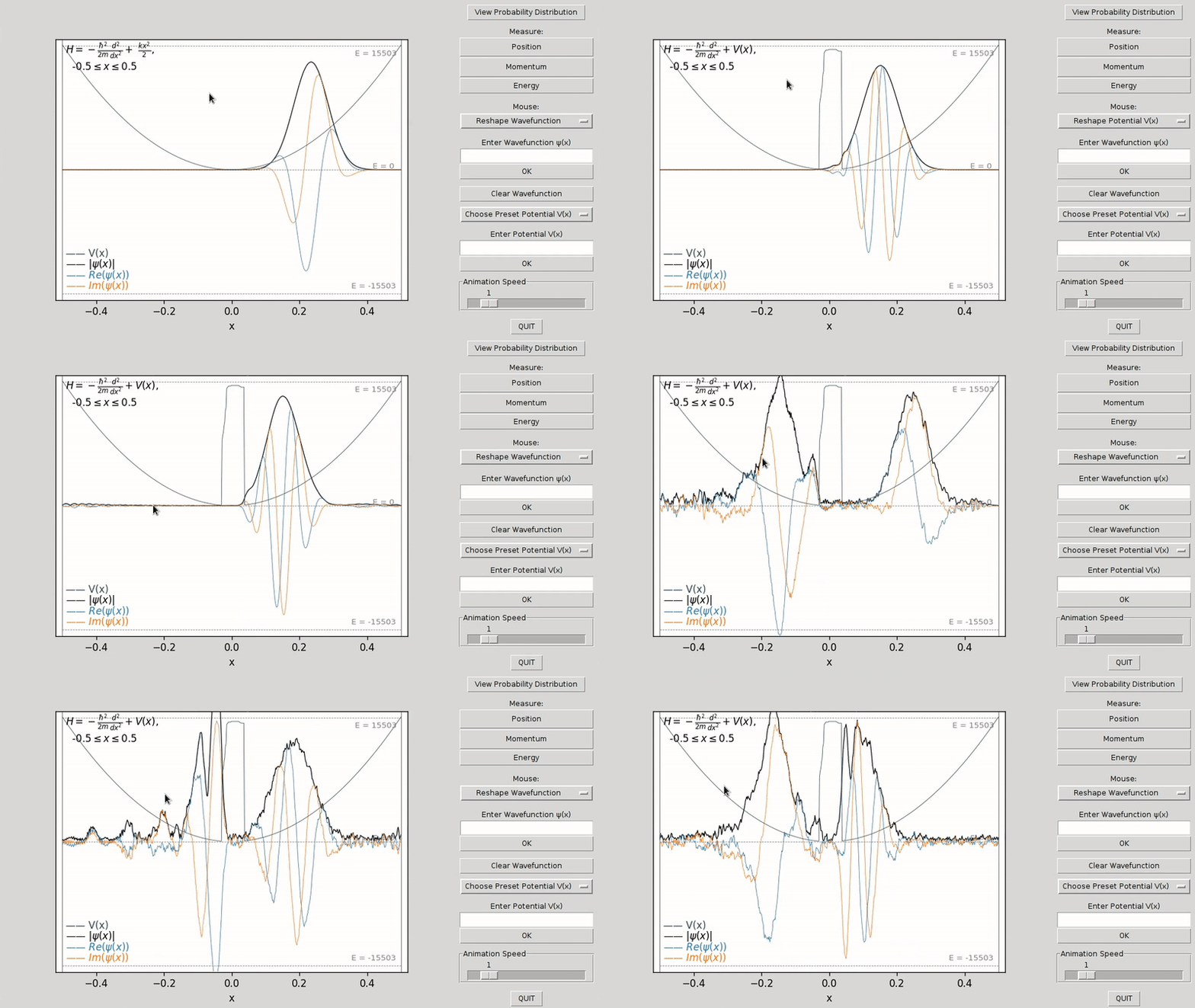
This program simulates a single quantum particle inside a bounded, shapeable 1D potential. The dynamics of this quantum particle are given by |ψ(t)> = U(t)|ψ(0)>, where t is time, |ψ> is the wavefunction vector ket of the particle, and U(t) is the unitary time evolution matrix. Numerical solutions to this equation may be found using the Crank-Nicolson method, which is derived in Exercise 9.8 of Mark Newmann's Computational Physics for the free particle case.
This project would not be possible without the following libraries: Numpy for numerical calculations, Sympy for symbolic computations, Matplotlib for graphing, and Tkinter for the GUI.
Make sure that you have at least Python 3.6.5 with Numpy, Matplotlib, Sympy and Scipy installed. Install these by running pip3 install numpy matplotlib sympy scipy. TKinter is also required and (on some Linux distributions) it can be installed with sudo apt-get install python3-tk. You may also optionally install Numba, which improves performance. To install Numba, run pip3 install numba.
Obtain all the necessary code by cloning this repository or downloading it, then run the file app.py. You should see something like:
The graph displays the wavefunction ψ(x) and the potential V(x). The top left corner displays a legend showing the Hamiltonian H of the system and its x-axis boundaries, which extend from -0.5 to 0.5. Note that the units on the x-axis and all other units of measurement are not in metric units, but in natural units, where all fundamental constants are set to one.
Use the mouse to draw a new shape for either the wavefunction ψ(x) or the potential V(x). To switch between reshaping the wavefunction or the potential, right click and select either Reshape Potential V(x) or Reshape Wavefunction.
The complex-valued wavefunction ψ(x) is not physically meaningful, but its probability density *ψ(x)ψ(x) is; switch to this view by clicking View Probability Distribution.
Measure observables by clicking on the Position, Momentum, and Energy buttons. To view their expectation values and standard deviations, right click and select Toggle Expectation Values.
To select a stationary state, first right click and select Select Energy Level. This presents a graphical view of each of the energy levels, where clicking on any one of these energy levels transforms the wavefunction into the corresponding energy eigenstate.
You can type in a new wavefunction ψ(x) in the Enter Wavefunction ψ(x) entry box. The wavefunction that you enter can depend on other additional variables aside from x, where new sliders will be created that allow you to manipulate the value of these additional variables. Note that the function ees(n, x) enters an energy eigenstate, where n specifies its energy level. You can also type and enter a new potential V(x) using the Enter Potential V(x) entry box. Just like for the wavefunction entry box, the potential that you enter here can depend on other additional variables aside from x, where new sliders will be created that allow you to manipulate these additional variables.
Use the Choose Preset Potential V(x) drop-down menu to select a preset potential V(x). To clear the wavefunction, press the Clear Wavefunction button. To alter the speed of the simulation, move the Animation Speed slider. To close the application, press QUIT.
To get a plain Matplotlib animation without any GUI, either directly run animation.py or import it separately. If you import it, make sure that you are running Matplotlib in interactive mode, and that you create an instance of QuantumAnimation. You can then measure observables by using its methods measure_energy(), measure_position(), and measure_momentum(). To switch between a view of the wavefunction itself or its probability density, use the methods display_probability() or display_wavefunction(). To change the wavefunction or potential, use set_wavefunction([new wavefunction]) and set_unitary([new_potential]), where new_wavefunction and new_potential can either be a string or a Numpy array.
The actual physics are contained in the classes Wavefunction1D and UnitaryOperator1D, which encapsulate the wavefunction and unitary operator. These are in the module qm.
For more content like this, have a look at the interactive quantum simulations written by Daniel Schroeder, Paul Falstad, and PhET Colorado. It were these simulations that inspired me to write my own in Python. Then have a look into the quantum mechanics module QuTiP, for a less GUI-based but more technical and in depth exploration of quantum mechanics. You may also want to try exercise 9.8 in the previously mentioned Computational Physics book by Mark Newman, as well as the other questions in this chapter.
Newman, M. (2013). Partial differential equations. In Computational Physics, chapter 9. CreateSpace Independent Publishing Platform.

