A modern robotic toolkit for localization and mapping -- reducing the barrier of entry for Simultaneous Localization and Mapping (SLAM).

Towards non-parametric / parametric state estimation and navigation solutions. Implemented in Julia (and JuliaPro) for a fast, flexible, dynamic and productive robot designer experience. This framework maintains good interoperability with other languages like C/C++ or Python, as listed in features below. Multi-modal (quasi-multi-hypothesis) navigation and mapping solutions, using various sensor data, is a corner stone of this package. Multi-sensor fusion is made possible via vertically integrated Multi-modal iSAM.

Critically, this package can operate in the conventional SLAM manner, using local dictionaries, or centralize around the FactorGraph through a graph database using CloudGraphs.jl, as discussed here[1]. A variety of plotting, 3D visualization, serialization, LCM middleware, and analysis tools come standard. Please see internal packages, Robot Motion Estimate RoME.jl and back-end solver IncrementalInference.jl.

Comments, questions and issues welcome.

Examples

Intersection of ambiguous elevation angle from planar SONAR sensor:

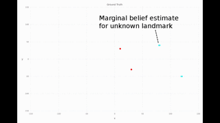
Bi-modal belief

Multi-session Turtlebot example of the second floor in the Stata Center:

Multi-modal range only example:

Installation

Requires via sudo apt-get install, see DrakeVisualizer.jl for more details.

libvtk5-qt4-dev python-vtk

Then install required Julia packages

julia> Pkg.add("Caesar")

Note that Database related packages will not be automatically installed. Please see section below for details.

Basic usage

Here is a basic example of using visualization and multi-core factor graph solving:

addprocs(2)
using Caesar, RoME, TransformUtils, Distributions

# load scene and ROV model (might experience UDP packet loss LCM buffer not set)
vc = startdefaultvisualization()
sc1 = loadmodel(:scene01); sc1(vc)
rovt = loadmodel(:rov); rovt(vc)


initCov = 0.001*eye(6); [initCov[i,i] = 0.00001 for i in 4:6];
odoCov = 0.0001*eye(6); [odoCov[i,i] = 0.00001 for i in 4:6];
rangecov, bearingcov = 3e-4, 2e-3

# start and add to a factor graph
fg = identitypose6fg(initCov=initCov)
tf = SE3([0.0;0.7;0.0], Euler(pi/4,0.0,0.0) )
addOdoFG!(fg, Pose3Pose3(MvNormal(veeEuler(tf), odoCov) ) )

visualizeallposes!(vc, fg, drawlandms=false)

addLinearArrayConstraint(fg, (4.0, 0.0), :x2, :l1, rangecov=rangecov,bearingcov=bearingcov)
visualizeDensityMesh!(vc, fg, :l1)
addLinearArrayConstraint(fg, (4.0, 0.0), :x1, :l1, rangecov=rangecov,bearingcov=bearingcov)

solveandvisualize(fg, vc, drawlandms=true, densitymeshes=[:l1;:x2])

Major features

• Performing multi-core inference with Multi-modal iSAM over factor graphs, supporting Pose2, Pose3, Point2, Point3, Null hypothesis, Multi-modal, KDE density, partial constraints, and more.

tree = wipeBuildBayesTree!(fg, drawpdf=true)
inferOverTree!(fg, tree)

• Or directcly on a database, allowing for separation of concerns

slamindb()

• Local copy of database held FactorGraph

fg = Caesar.initfg(cloudGraph, session)
fullLocalGraphCopy(fg)

• Saving and loading FactorGraph objects to file

savejld(fg, file="test.jld", groundtruth=gt)
loadjld(file="test.jld")

• Visualization through MIT Director.

visualizeallposes(fg) # from local dictionary
drawdbdirector()      # from database held factor graph

• Foveation queries to quickly organize, extract and work with big data blobs, for example looking at images from multiple sessions predicted to see the same point [-9.0,9.0] in the map:

neoids, syms = foveateQueryToPoint(cloudGraph,["SESS21";"SESS38";"SESS45"], point=[-9.0;9.0], fovrad=0.5 )
for neoid in neoids
    cloudimshow(cloudGraph, neoid=neoid)
end

• Operating on data from a thin client processes, such as a Python front-end examples/database/python/neo_interact_example.jl

• A caesar-lcm server interface for C++ applications is available here.

• A multicore Bayes 2D feature tracking server over tcp

julia -p10 -e "using Caesar; tcpStringBRTrackingServer()"

And many more, please see the examples folder.

Dependency Status

Major Dependencies	Status	Test Coverage
Caesar.jl
RoME.jl
IncrementalInference.jl
KernelDensityEstimate.jl
TransformUtils.jl
DrakeVisualizer.jl

Database interaction layer

For using the solver on a Database layer, you simply need to switch the working API. This can be done by calling the database connection function, and following the prompt:

using Caesar
backend_config, user_config = standardcloudgraphsetup()
fg = Caesar.initfg(sessionname=user_config["session"], cloudgraph=backend_config)
# and then continue as normal with the fg object, to add variables and factors, draw etc.

If you have access to Neo4j and Mongo services you should be able to run the four door test.

Go to your browser at localhost:7474 and run one of the Cypher queries to either retrieve

match (n) return n

or delete everything:

match (n) detach delete n

You can run the multi-modal iSAM solver against the DB using the example MM-iSAMCloudSolve.jl:

$ julia -p20
julia> using Caesar
julia> slamindb() # iterations=-1

Database driven Visualization can be done with either MIT's MIT Director (prefered), or Collections Render which additionally relies on Pybot. For visualization using Director/DrakeVisualizer.jl:

$ julia -e "using Caesar; drawdbdirector()"

And an example service script for CollectionsRender is also available.

Contributors

D. Fourie, S. Claassens, P. Vaz Teixeira, N. Rypkema, S. Pillai, R. Mata, M. Kaess, J. Leonard

Future targets

This is a work in progress package. Please file issues here as needed to help resolve problems for everyone!

Hybrid parametric and non-parametric optimization. Incrementalized update rules and properly marginalized 'forgetting' for sliding window type operation. We defined interprocess interface for multi-language front-end development.

References

[1]  Fourie, D., Claassens, S., Pillai, S., Mata, R., Leonard, J.: "SLAMinDB: Centralized graph
     databases for mobile robotics" IEEE International Conference on Robotics and Automation (ICRA),
     Singapore, 2017.