Quantum Kite is a multi threaded C++ package for efficient evaluation of spectral properties of large-scale tight-binding (TB) hamiltonians. In this tutorial, we will present the code functionalities through different examples in form of inline codes and gists that you can simply copy or download from our Github page and run. For a detailed information on the method behind the package, we suggest you to take a look at the section Resources. If you find a problem, a bug, or have any further question, we encourage you to contact us.
The code is divided in three different layers. The starting point, which is the interface between the user and the C++ code, is based on a Python script. At this level, the definition of a TB model uses Pybinding, a python package to study TB hamiltonians. In the next sections we will introduce basic functionalities of the Pybinding package, which will be used to build the model and the basic funcionalities of Kite. For more advanced examples you can check https://quantum-kite.com/category/examples/.
Quantum Kite is shipped as a source code that can be compiled following the instruction provided in the section Installation . The package contains a the transport code and also a post-processing code. The interconnection between different parts of the package is done using the Hierarchical Data Format (HDF5 package). The model is built with a python script and it is exported, together with the calculation settings, to a *.h5 file, which is used later as a TB input to Quantum Kite. All the output data of the simulation is saved in the same *h5 file that is finally posprocessed by posprocessing tools that produce different *.dat files for the calculated quantities.
In short, the code workflow is the following:
- Use a python script to build and export a TB model from Pybinding and define the settings for Quantum Kite.
- Run Quantum Kite with a defined TB model.
- Run post-processing tools.
- Visualise the data.
Before going to the examples, let's see how to load Pybinding.
If all the installation requirements are fulfilled, Pybinding package can be imported in the python script. In all the scripts of this tutorial, the required packages will be included with the following aliases:
import pybinding as pb
import numpy as np
import matplotlib.pyplot as plt
If you want to use pybinding predefined styles for visualization of the lattice, you can simply write:
pb.pltutils.use_style()inside the script.
The most important object for building a TB model is pb.Lattice, which carries the full information about the unit cell (position of lattice sites, sublattices, orbitals, lattice vectors and hopping parameters). These are the input parameters for the Lattice. Pybinding also provide additional features based on the real-space information, as for example, the reciprocal vectors and the Brillouin zone.
To ilustrate how the python script works, let us make a simple square lattice with a single lattice site.
First, import all the packages:
import pybinding as pb
import numpy as np
import matplotlib.pyplot as plt
The following syntax can be used to define the lattice vectors that build the regular lattice:
a1 = np.array([1,0]) # [nm] define the first lattice vector
a2 = np.array([0, 1]) # [nm] define the second lattice vector

lat = pb.Lattice(a1=a1, a2=a2) # define a lattice object
Now we can add the desired lattice sites inside the unit:
lat.add_sublattices(
    # make a lattice site (sublattice) with a tuple
    # (name, position, and onsite potential)
    ('A', [0, 0], onsite[0])
)
and add the hoppings between the neighboring sites:
lat.add_hoppings(
    # make an hopping between lattice site with a tuple
    # (relative unit cell index, site from, site to, hopping energy)
    ([1, 0], 'A', 'A', - 1 ),
    ([0, 1], 'A', 'A', - 1 )
)
The relative unit cell index [n, m] is a parameter of the unit cell
(in the notation n * a1 , m * a2) to which the hopping occurs. The index
[0, 0] is a reference hopping inside the unit cell, while other indexes mark
the periodic hopping.
It's important to emphasize that by adding the hopping (i, j) between sites i and j, the hopping term (j, i) is added automatically and it is not allowed to add them twice. Also, it is not allowed to add a hopping(i, i) inside the cell [0,0] because these terms are actually onsite energies that can be added when adding a lattice site (sublattice).
Now we can plot the lattice:
lat.plot()
plt.show()
or visualize the Brillouin zone:
lat.plot_brillouin_zone()
plt.show()
We can try to build a slightly advanced example,like a graphene lattice.
For more advanced examples and pre-defined lattices, please refere to pybinding documentation.
It is possible to incorporate different types of disorder, including a variety of onsite and bond disorders. This is covered in a specific tutorial with more advanced examples, as it is not a necessary part of the script.
After making the lattice object, we export the model and the information about the quantities that we want to calculate to a hdf file. For this, we need additional functionalities provided by kite that can be imported with:
from kite_config import Configuration, Calculation, Modification, Disorder, StructuralDisorder, \
    export_lattice, make_pybinding_model
In this script, three different classes are defined:
ConfigurationCalculationModification
These three classes provide all the information about the system that is used in the calculation and also the quantities we want to calculate.
The objects of class Configuration carry the info about:
-
divisions- integer number that defines the number of decomposition parts in each direction. This divides the lattice into various sections that are computed in parallel.nx = ny = 2
This decomposition allows a great speed up of the calculation that scales with the the number of decomposed parts. We recommend its usage. However, the product of the values of nx and ny is the number of threads that the code uses. It cannot exceed the number of cores available in your computer. One must also notice that it is not efficient to decompose small systems with lateral sizes smaller than 128 unit cells of a normal lattice.
-
length- integer number of unit cells along the direction of lattice vectors:lx = 256 ly = 256
The lateral size of the decomposed parts are given by lx/nx and ly/ny that need to be integer numbers.
-
boundaries- boolean value defining periodic boundaries along each direction. True for periodic boundary conditions, and False for open boundary conditions. For now, Kite only accepts periodic boundary conditions. -
is_complex- boolean value that defines whether the Hamiltonian is complex or not. For optimisation purposes, Kite only considers and stores complex data with the setting is_complex=True. False indicates real values. -
precision- integer identifier of data type that the system uses. For optimisation purposes, kite also allows the user to define the precision of the calculation. Use 0 for float, 1 for double, and 2 for long double. -
Chebyshev expansions need renomalized hamiltonians where the energy spectrum is bounded [-1,1]. Our interface provides an automated scaling. However, if you want to define the bounds of your hamiltonian by hand, you can useIf you need more details about this point, refere to Resources where we discuss the method in details.
As a result, a Configuration object is structured in the following way:
configuration = ex.Configuration(divisions=[nx, ny], length=[lx, ly], boundaries=[True, True], is_complex=False, precision=1)Finally it is time to write the Calculation object that carries out the information about the quantities that are going to be calculated. For this part, we still need to include more paramenters, related to the Chebyshev expansion (our examples already have optimized parameters for a normal desktop computer). All quantities need the following parameters:
-
num_moments defines the number of moments of the Chebyshev expansion. This number can be varied, dependening on the energy resolution you expect. Tipically we use **num_moments>max(lx,ly) **, so it should scales with the size of your system. However, the optimal number depends on the lattice. The user should also avoid an excessive number of moments that exceed the desired energy resolution. Otherwise the calculation will begin to converge to the discrete energy levels of the finite system. We professional usage, we suggest a convergence analysis in function of the number of polynomials used in the expansion.
-
num_random defines the number of random vectors involved in the stochastic calculation of quantities (for more details, see Resources). This number also depends of the size of the system. For large systems that are self-averaged, it can be very small. For professional usage, we suggest a convergence analysis in function of the number of random vectors.
-
num_disorder defines the number of disorder realisations, useful for disordered systems.
The other parameters that are specific for each quantity are explained after the function definitions
Here we list features/functions that are available at the moment:
-
fname - name of the function that you want to evaluate, case insensitive:
dos- density of states. Other parameter:num_pointsis the number of points the in energy axis that is going to be used by the post-processing tool to output the density of states.conductivity_optical- optical conductivity linear response, parameters:direction,temperature,num_pointsconductivity_dc- zero frequency conductivity linear response, parameters:direction,temperature,num_pointsconductivity_optical_nonlinear- zero frequency conductivity in linear response, parameters:direction,temperature,num_pointssingleshot_conductivity_dc- single energy zero frequency longitudinal conductivity (zero temperature), parameters:direction(limited to longitudinal direction),energy,gamma.
The following parameters are optional and are available for a function that supports them, for more info check previous definitions of function names:
-
direction- direction along which the conductivity is calculated (longitudinal: 'xx', 'yy', transversal: 'xy', 'yx') -
temperaturea temperature in Fermi Dirac distribution that is used for the calculation of optical and DC conductivities. -
num_pointsis the number of points the in energy axis that is going to be used by the post-processing tool to output the density of states. -
special- simplified form of nonlinear optical conductivity hBN example -
energy- selected value of energy at which we want to calculate the singleshot_conductivity_dc -
gamma- Imaginary term in the denominator of the Green function that provides a controled broadening [eV] (for technical details, see Resources).
As a result, calculation is structured in the following way:
calculation = Calculation(configuration)

calculation.dos(num_points=1000, num_random=10, num_disorder=1, num_moments=512)

calculation.conductivity_optical(num_points=1000, num_random=1, num_disorder=1, num_moments=512, direction='xx')

calculation.conductivity_dc(num_points=1000, num_moments=256, num_random=1, num_disorder=1,direction='xy', temperature=1)

calculation.singleshot_conductivity_dc(energy=[(n/100.0 - 0.5)*2 for n in range(101)], num_moments=256, num_random=1, num_disorder=1,direction='xx', gamma=0.02)

calculation.conductivity_optical_nonlinear(num_points=1000, num_moments=256, num_random=1, num_disorder=1,direction='xxx', temperature=1.0, special=1)
Important: the user can decide what functions are used in a calculation. However, it is not possible to provide the same function twice with different paramenters. The code only accepts one defined function for each hdf file. One should generate different hdf files if a same function with different paramenters is needed.
The last object of a class Modification defines special modifiers. At the moment, only magnetic_field is available as an optional integer parameter, which if defined as 1 adds the minimal value of the magnetic field that obeys a commensurability condition between the magnetic unit cell and the material unit cell
It can be defined as:
modification = ex.Modification(magnetic_field=1)Finally, it is time to export all the settings to a hdf5 that is the input for Kite:
When these objects are defined, we can export the file that will contain set of input instructions for Quantum Kite:
kite.export_lattice(lattice, configuration, calculation, modification, 'test.h5')The following organizes all the instructions in a single file:
https://gist.github.com/quantum-kite/19472b95b0348a161b8987137ea7e063
To run the code and the postprocess it, use
./KITEx test.h5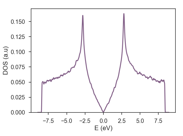
./postprocessing/tools/kitepos test.h5After calculating the quantity of interest and post-processing the data, we can plot the resulting data with the following script:
https://gist.github.com/quantum-kite/9a935269845eae3f8590f364be12cb49
If you want to make these steps more automatic, you can use the following Bash script
https://gist.github.com/quantum-kite/c002610a4d43a478cf0f967129f97da7.