differentially-expressed-genes.Rmd

---
title: "Differentially Expressed Genes Network Analysis"
author: "Kozo Nishida, Kristina Hanspers and Alex Pico"
date: "`r Sys.Date()`"
output:
  BiocStyle::html_document:
    toc: true
    toc_depth: 4
    df_print: paged
---
```{r, echo = FALSE}
knitr::opts_chunk$set(
  eval=FALSE
)
```

*The R markdown is available from the pulldown menu for* Code *at the upper-right, choose "Download Rmd", or [download the Rmd from GitHub](https://raw.githubusercontent.com/nrnb/gsod2019_kozo_nishida/master/differentially-expressed-genes.Rmd).*

<hr />

This protocol describes a network analysis workflow in Cytoscape for a set of differentially expressed genes. Points covered:

- Retrieving relevant networks from public databases
- Network functional enrichment analysis
- Integration and visualization of experimental data
- Exporting network visualizations

<center>
![](https://cytoscape.org/cytoscape-tutorials/protocols/differentially-expressed-genes/string-ovarian-drivers.png)
</center>

<hr />

# Installation
```{r, eval = FALSE}
if (!requireNamespace("BiocManager", quietly = TRUE))
  install.packages("BiocManager")

if(!"RCy3" %in% installed.packages())
  BiocManager::install("RCy3")

library(RCy3)
```

# Getting started
First, launch Cytoscape and keep it running whenever using RCy3. Confirm that you have everything installed and running:
```{r}
    cytoscapePing()
    cytoscapeVersionInfo()
```

# Prerequisites

If you haven't already, install the [STRINGapp](http://apps.cytoscape.org/apps/stringapp)

```{r}
installApp('stringApp')
installApp('yFiles Layout Algorithms')
```

# Background

Ovarian serous cystadenocarcinoma is a type of epithelial ovarian cancer which accounts for ~90% of all ovarian cancers.
The data used in this protocol are from [The Cancer Genome Atlas](https://cancergenome.nih.gov/), in which multiple subtypes of serous cystadenocarcinoma were identified and characterized by mRNA expression.

We will focus on the differential gene expression between two subtypes, **Mesenchymal** and **Immunoreactive**.

For convenience, the data have already been analyzed and pre-filtered, using log fold change value and adjusted p-value.

# Network Retrieval

Many public databases and multiple Cytoscape apps allow you to retrieve a network or pathway relevant to your data.
For this workflow, we will use the STRING app. Some other options include:

- [WikiPathways](https://nrnb.org/gsod2019_kozo_nishida/html_documents/Rmd/wikipathways-app.html)
- [NDEx](http://www.ndexbio.org/)
- [GeneMANIA](https://genemania.org/)

# Retrieve Networks from STRING

To identify a relevant network, we will query the STRING database in two different ways:

- Query **STRING protein** with the list of differentially expressed genes.
- Query **STRING disease** for ovarian cancer.

## STRING Protein Query: Up-regulated genes

- Load the file containing the list of up-regulated genes, TCGA-Ovarian-MesenvsImmuno_UP.txt:

```{r}
df <- read.table("https://cytoscape.github.io/cytoscape-tutorials/protocols/data/TCGA-Ovarian-MesenvsImmuno_UP.txt")
```

- We will use the identifiers in the first column of this datafile to run a **STRING protein query**, with confidence (score) cutoff of 0.4:

```{r}
string.cmd = paste('string protein query query="', paste(df$V1, collapse = '\n'), '" cutoff=0.4  species="Homo sapiens"', sep = "")
commandsRun(string.cmd)
```

The resulting network will load automatically.

![](images/string-up.png)

The resulting network contains up-regulated genes recognized by STRING, and interactions between them with an evidence score of 0.4 or greater.

```{r}
getTableColumnNames('edge')
```

```{r}
evidence.score <- getTableColumns('edge', "stringdb::score")
min(evidence.score)
```

# Enrichment Analysis Options

Next, we are going to perform enrichment anlaysis uing the STRING app.
Note that there are several other options, including:

- [clusterProfiler](http://bioconductor.org/packages/release/bioc/vignettes/clusterProfiler/inst/doc/clusterProfiler.html): An R package for ORA and GSEA
- [g-Profiler](https://biit.cs.ut.ee/gprofiler/): An enrichment analysis website
- [EnrichR](http://amp.pharm.mssm.edu/Enrichr/): A website that performs enrichment against dozens of ontologies and pathway resources
- [ClueGO](http://apps.cytoscape.org/apps/cluego): Creates and visualizes a functionally grouped network of terms/pathways
- [BiNGO](http://apps.cytoscape.org/apps/bingo): GO overrepresentation analysis on networks
- [EnrichmentMap](https://cytoscape.org/cytoscape-tutorials/protocols/enrichmentmap-pipeline/): Visualize the results of gene-set enrichment as a network

## STRING Enrichment

The STRING app has built-in enrichment analysis functionality, which includes enrichment for GO Process, GO Component, GO Function, InterPro, KEGG Pathways, and PFAM.

- First, we will run the enrichment on the whole network, against the genome: 

```{r}
string.cmd = 'string retrieve enrichment allNetSpecies="Homo sapiens", background=genome  selectedNodesOnly="false"'
commandsRun(string.cmd)
string.cmd = 'string show enrichment'
commandsRun(string.cmd)
```

- When the enrichment analysis is complete, a new tab titled **STRING Enrichment** will open in the **Table Panel**.

![](images/string-enrichment.png)

The STRING app includes several options for filtering and displaying the enrichment results.
The features are all available at the top of the **STRING Enrichment** tab.

- We are going to filter the table to only show GO Process. 

```{r}
string.cmd = 'string filter enrichment categories="GO Process", overlapCutoff = "0.5", removeOverlapping = "true"'
commandsRun(string.cmd)
```

- Next, we will add a split donut chart to the nodes representing the top terms by clicking on ![](images/ChartIcon.png).

```{r}
string.cmd = 'string show charts'
commandsRun(string.cmd)
```

![](images/string-enrichment-chart.png)

## STRING Protein Query: Down-regulated genes

- Repeat the network search, enrichment analysis and visualization for the set of down-regulated genes by using the first column of [TCGA-Ovarian-MesenvsImmuno_DOWN.txt](https://cytoscape.github.io/cytoscape-tutorials/protocols/data/TCGA-Ovarian-MesenvsImmuno_DOWN.txt):

```{r}
df <- read.table("https://cytoscape.github.io/cytoscape-tutorials/protocols/data/TCGA-Ovarian-MesenvsImmuno_DOWN.txt")
string.cmd = paste('string protein query query="', paste(df$V1, collapse = '\n'), '" cutoff=0.4  species="Homo sapiens"', sep = "")
commandsRun(string.cmd)
```

Now we can perform STRING Enrichment analysis on the resulting network.

```{r}
string.cmd = 'string retrieve enrichment allNetSpecies="Homo sapiens", background=genome  selectedNodesOnly="false"'
commandsRun(string.cmd)
string.cmd = 'string show enrichment'
commandsRun(string.cmd)
```

Filter the analysis results for non-redundant GO Process terms only, add split donut charts. To distinguish between the visualizations of up- and down-regulated results, pick a different color palette under Change Color Palette under Settings.

```{r}
string.cmd = 'string filter enrichment categories="GO Process", overlapCutoff = "0.5", removeOverlapping = "true"'
commandsRun(string.cmd)
```

```{r}
string.cmd = 'string show charts'
commandsRun(string.cmd)
```

## STRING Disease Query

Now, we will query the **STRING disease** database to retrieve a network of ovarian cancer associated genes, completely independent of our dataset.

```{r}
string.cmd = 'string disease query disease="ovarian cancer"'
commandsRun(string.cmd)
```

This will bring in the top 100 ovarian cancer associated genes connected with a confidence score greater than 0.4.
(We did not give them as parameters[100 and 0.4]. This is because the default values are those.)

# Data integration

Next we will import log fold changes and p-values from our TCGA dataset and use them to create a visualization.
Since the network and data use different identifiers, we first have to do some quick identifier mapping. 
In this case, we will use the gene symbol in the **display name** column to retrieve **Entrez Gene** identifiers.

```{r}
getTableColumnNames('node')
```


```{r}
mapped.cols <- mapTableColumn("display name",'Human','HGNC','Entrez Gene')
```

Here we set **Human** as species, **HGNC** as **Map from**, and **Entrez Gene** as **To**.

```{r}
head(mapped.cols)
```

`mapped.cols` displays a report of how many identifiers were mapped. Make note of this information as it impacts all down-stream analysis; If the mapping was unsuccessful, downstream analysis will be as well. You will notice the new column `Entrez Gene` in the Node Table.

```{r}
tail(getTableColumnNames('node'))
```

Next, we can load the data (a local copy of [TCGA-Ovarian-MesenvsImmuno_data.csv](https://cytoscape.github.io/cytoscape-tutorials/protocols/data/TCGA-Ovarian-MesenvsImmuno_data.csv)):

```{r}
df <- read.csv("https://cytoscape.org/cytoscape-tutorials/protocols/data/TCGA-Ovarian-MesenvsImmuno_data.csv")
```

```{r}
head(df)
```

We are now ready to integrate the data with the network (node) table in Cytoscape.
For importing the data we will use the following mapping: 

- **Key Column for Network** should be **Entrez Gene**.
- **Gene** should be the key of the data(`df`).

```{r}
loadTableData(df, data.key.column = "Gene", table = "node", table.key.column = "Entrez Gene")
```

You will notice two new columns (logFC and FDR.adjusted.Pvalue) in the Node Table. 

```{r}
tail(getTableColumnNames('node'))
```

# Visualization

We can now use the integrated data to create a network visualization.

- For node **Fill Color**, create a continuous mapping for **logFC**, with the following blue-red gradient. 

- First we have to remove the current mapping for node fill color:

```{r}
getVisualStyleNames()
```

```{r}
deleteStyleMapping("STRING style v1.5 - ovarian cancer", "NODE_FILL_COLOR")
```

- Next, we need the min and max of the **logFC** column:

```{r}
logFC.table <- getTableColumns('node', 'logFC')
```

```{r}
logFC.min <- min(logFC.table, na.rm = T)
logFC.max <- max(logFC.table, na.rm = T)
logFC.center <- logFC.min + (logFC.max - logFC.min)/2
```

- Let's create the mapping: 

```{r}
setNodeFontSizeDefault(4)
setNodeColorMapping('logFC', c(logFC.min, logFC.center, logFC.max), c('#0000FF', '#FFFFFF', '#FF0000'), style.name ="STRING style v1.5 - ovarian cancer")
```

- Change the default node **Fill Color** to light grey.

```{r}
setNodeColorDefault('#D3D3D3', style.name ="STRING style v1.5 - ovarian cancer")
```

_Pro-tip: If you apply the **yFiles Organic** layout, you can end up with network views like this..._
([**yFiles** Layout Algorithms App](http://apps.cytoscape.org/apps/yfileslayoutalgorithms) does not support any automation. Please select it in Cytoscape Desktop menubar.)

![](images/string-ovarian-styled.png)

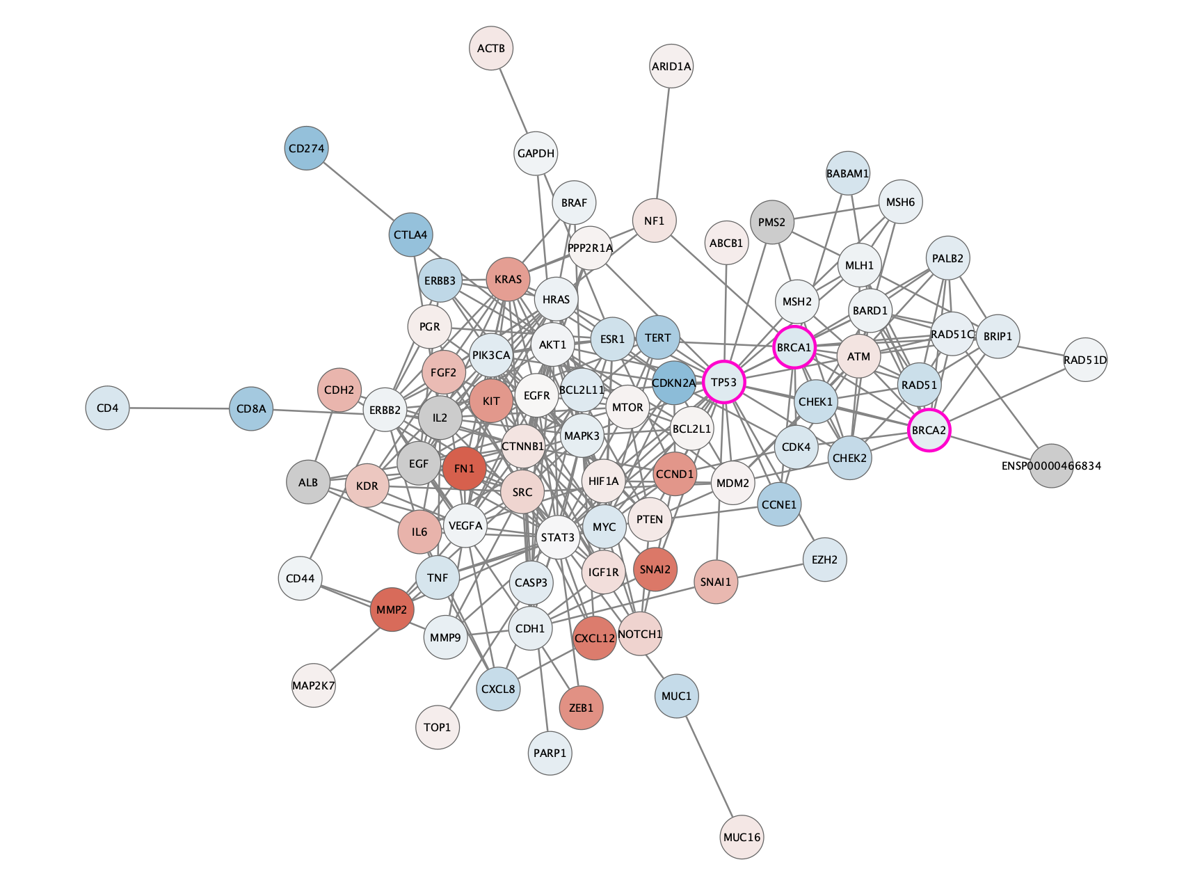
The TCGA found several genes that were commonly mutated in ovarian cancer, so called "cancer drivers".
We can add information about these genes to the network visualization, by changing the visual style of these nodes.
Three of the most important drivers are **TP53**, **BRCA1** and **BRCA2**.
We will add a thicker, clored border for these genes in the network.

- Select all three driver genes by:

```{r}
selectNodes(c("TP53", "BRCA1", "BRCA2"), by.col = "display name")
```

- Add a style bypass for node **Border Width** (5) and node **Border Paint** (bright pink):

```{r}
setNodeBorderWidthBypass(getSelectedNodes(), 5)
setNodeBorderColorBypass(getSelectedNodes(), '#FF007F')
```

The network will now look like this:

![](images/string-ovarian-drivers.png)

# Other Analysis Options

- Exploring networks: finding paths, hubs and modules (clusterMaker, MCODE, jActiveModules, NetworkAnalyzer, PathFinder)
- Extending networks with Transcription Factors, miRNAs, etc using CyTargetLinker

# Exporting Networks
Cytoscape provides a number of ways to export results and visualizations:

- As an image:

```{r}
exportImage('./differentially-expressed-genes', 'PDF')
exportImage('./differentially-expressed-genes', 'PNG')
exportImage('./differentially-expressed-genes', 'JPEG')
exportImage('./differentially-expressed-genes', 'SVG')
exportImage('./differentially-expressed-genes', 'PS')
```

- To a public repository:

```
exportNetworkToNDEx("user", "password", TRUE)
```

- As a Cytoscape JSON file:

```{r}
exportNetwork('./differentially-expressed-genes', 'cyjs')
```